Data modeling 101
Embeddable uses a data modeling layer to define and manage access to your data.
TL;DR
- A data modeling layer takes data requests from charts and components on your dashboard and turns them into SQL that is run against your database(s).
- It is a single source of truth for what SQL to generate based on the data request (as well as database type, data models and security context) you provide it.
- Defining data models is simple once you get your head around a few fundamental concepts.
What is a data modeling layer?
A data modeling layer is an abstraction layer that sits between the raw data in your databases and your analytics, defining data in clear, consistent terms that users understand. It is effectively a single source of truth for your data and metrics.
Using a data modeling layer (as opposed to writing each and every query, by hand, in SQL) comes with a number of significant advantages, particularly for customer-facing analytics:
- Consistency. No more worrying about whether all SQL queries on your dashboards are using the same consistent definition for a particular metric - you can be confident that the same definition is being used everywhere.
- Maintainability. If the definitions of your metrics change, or your data changes (which it will…), you only need to update your models in one single place (not dig through and update dozens, if not hundreds of hand-written SQL queries).
- Speed. You, or your non-technical teammates, can slice and dice and filter your data within Embeddable in just a few clicks, without having to write a single line of SQL, and you can be confident that the generated SQL will be optimized to perform well on your particular database.
How is it used within Embeddable?
In Embeddable the data modeling layer is essential for loading data from your databases into your charts. It is responsible for generating the SQL that will run against your database:
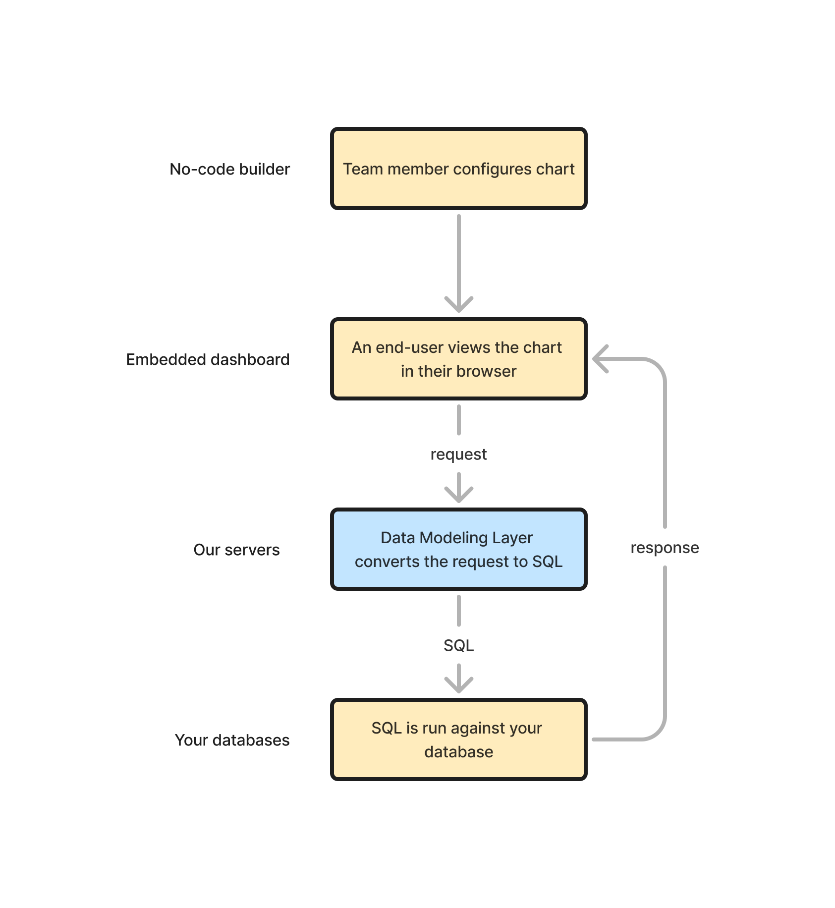
Team member configures chart
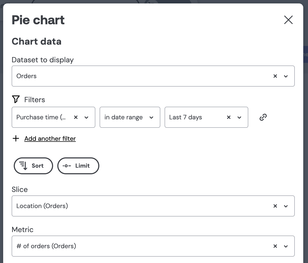
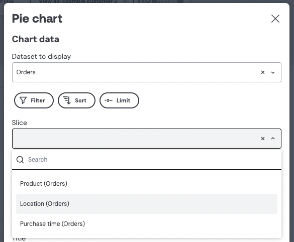
Firstly, in order for a user to see a chart in your embedded Embeddable dashboard, it has to be added to a dashboard in Embeddable’s no-code dashboard builder. E.g. a Pie Chart may be configured, as shown below, to show # of orders, purchased in the Last 7 days, sliced by Location:
An end-user views the chart in their browser
This Pie Chart will now show up on the embedded dashboard for the end-user, but before it can render, it first it needs to load its data:

So, what the chart will do (while showing a loading spinner like above) is use the configuration provided in Step 1 (above) to request data from the Embeddable servers. Such a request may look something like this:
{
    "query": {
        "dimensions": [
            "orders.location"
        ],
        "measures": [
            "orders.count"
        ],
        "timeDimensions": [
            {
                "dimension": "orders.created_at",
                "dateRange": "Last 7 days"
            }
        ],
        "limit": 100
    }
}
Data modeling layer converts the request to SQL
This is where the data modeling layer comes in. The data modeling layer will take that request and convert it into the correct SQL for your database (and how exactly it does this we’ll explain below).
The generated SQL may look something like this:
SELECT
  CONCAT(city, ', ', country) "orders__location",
  count("orders".id) "orders__count"
FROM
  public.orders AS "orders"
WHERE
  (
    "orders".created_at >= '2025-02-25T00:00:00.000Z'::timestamptz
    AND "orders".created_at <= '2025-03-03T23:59:59.999Z'::timestamptz
  )
GROUP BY
  1
ORDER BY
  2 DESC
LIMIT
  100
SQL is run against your database
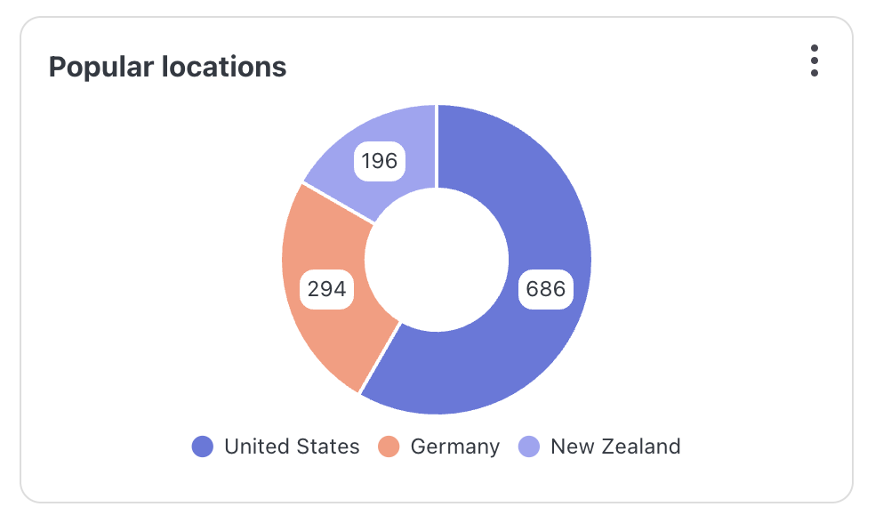
This SQL is then run against your database, the results are returned to the Pie Chart, and the Pie Chart can render itself in all its glory.
The returned results might look something like this:
{
    "result":
    [
        {
            "orders.location": "Los Angeles, United States",
            "orders.count": "686"
        },
        {
            "orders.location": "Hamburg, Germany",
            "orders.count": "294"
        },
        {
            "orders.location": "Christchurch, New Zealand",
            "orders.count": "196"
        }
    ],
    "durationMs": 190
}
And the final rendered Pie Chart might then look like this:
How does it generate SQL?
But how does the data modeling layer know what SQL to generate given a particular request?
Going back to our original flow diagram you can see that a data modeling layer is simply a box that takes a request as input and spits out SQL:
In practice there is a little more to it. A data modeling layer also has three other important inputs it uses when deciding what SQL to generate:
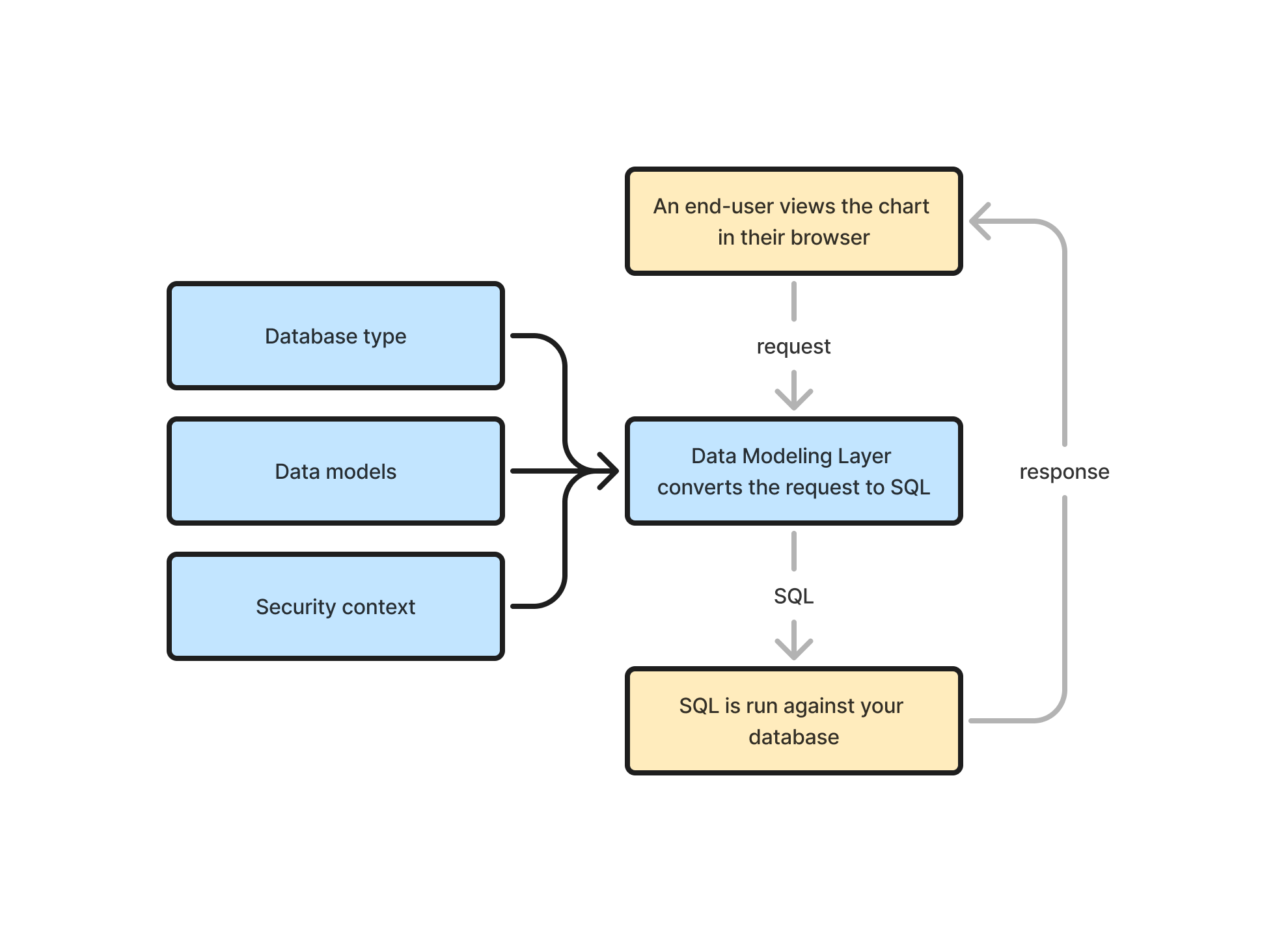
- Database type: in Embeddable this is defined by the type of the database connection you set up and it tells the data modeling layer whether to, for example, generate SQL in the Postgres, MySQL or Snowflake dialect (many other dialects supported). This is important to the data modeling layer as different databases have slightly different syntax for different query constructs (as a simple example, Postgres surrounds table names with “double quotes”, whereas MySQL uses `backticks`).
- Security context: this is just a simple set of key-value pairs (e.g.
{ "user_id": 1534 }) that you pass to Embeddable when generating a security token to load a dashboard in your application. It provides the necessary information for row-level security to be applied. E.g. theuser_idin this example may be used by the data modeling layer to apply aWHERE user_id = 1534filter to the generated SQL, ensuring that the end user only ever sees the data rows that they are allowed to see (learn more about how row-level security works in Embeddable here). - Data models: this is where the magic happens. Data models are simple files, defined by you, that give the data modeling layer all the context it needs to know in order to generate the correct SQL for your data. The remainder of this page will take you through a simple example data model.
Data models
Data models are the building blocks that power the data modeling layer.
Under the hood, Embeddable uses a popular data modeling language called Cube (opens in a new tab). We use it because it is very simple to learn, but is also very powerful and flexible.
Let’s look at an example.
A simple example
Suppose we have an orders table in our database like so:
| id | product | city | country | created_at | price_usd |
|---|---|---|---|---|---|
| 1 | Eggs | Los Angeles | United States | 2025-03-01 | 3.79 |
| 2 | Milk | Christchurch | New Zealand | 2026-08-27 | 4.60 |
We could define a data model for it, in an orders.cube.yml file like so:
cubes:
  - name: orders
    sql_table: public.orders

    measures:
      - name: count
        type: count
        title: '# of orders'

      - name: total_price
        title: "Total USD"
        type: sum
        sql: price_in_cents / 100.0

    dimensions:
      - name: id
        sql: id
        type: number
        primary_key: true
        public: false

      - name: created_at
        title: "Purchase time"
        sql: created_at
        type: time

      - name: product_name
        title: 'Product'
        sql: product
        type: string

      - name: location
        sql: CONCAT(city, ', ', country)
        type: string
Data modeling may seem slightly daunting at first, but there’s just a few simple concepts to understand and then you know everything you need to know.
Things to notice:
- The
nameof the cube is just a unique name we want to give to our model (doesn’t need to match the name of the table).cubes: - name: orders - The
sql_tabletells our data modeling layer (Cube) which table to use in theFROMclause when generating the SQL, e.g.SELECT ... FROM public.orders ....sql_table: public.orders - The
measuresare the metrics we want to be able to calculate (count,sum,count_distinct,max,minetc.). You can expect to see these in theSELECTandHAVINGclauses of the generated SQL. E.g.SELECT sum(price_in_cents / 100.0)measures: - name: count type: count title: '# of orders' - name: total_price title: "Total USD" type: sum sql: price_in_cents / 100.0 - The
dimensionsare the virtual columns that we want to expose to the Embeddable dashboard builderdimensions: - name: id sql: id type: number primary_key: true public: false - name: created_at title: "Purchase time" sql: created_at type: time - E.g. the product_name dimension has its
sqlparameter defined asproductwhich simply means that if the product_name is requested by a chart, then thatsqlwill be used in the generated SQL, e.g.SELECT product FROM public.orders.- name: product_name title: 'Product' sql: product type: string - Whereas the location dimension has its
sqldefined asCONCAT(city, ‘, ‘, country). This means exactly the same. If location is requested, then thatsqlwill be used in the generated SQL, e.g.SELECT CONCAT(city, ', ', country) from public.orders.- name: location sql: CONCAT(city, ', ', country) type: string - You can also expect to see these dimensions appear in the
GROUP BYandWHEREclauses of the generated SQL, e.g.GROUP BY CONCAT(city, ', ', country)orWHERE product = 'Ice cream'
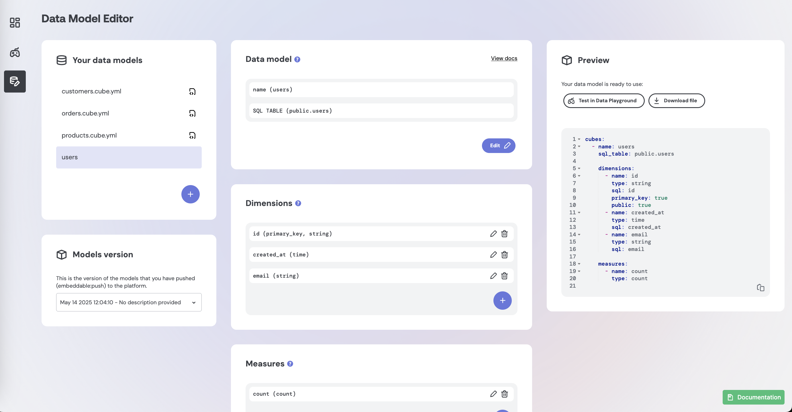
The easiest way to get started with data modeling is to use Embeddable's in-platform Data Model Editor which guides you through creating your models in a step-by-step UI:
And then test your models using Embeddable's Data Playground:
How it all fits together
Let’s go back to our Pie Chart configuration screen from earlier. The reason Product, Location and Purchase time are even available inside Embeddable to choose from is because you’ve defined them in the data model:
Once you’ve defined your first data model, you just need to push it to your Embeddable workspace (learn how). As soon as you’ve done that you will now automatically be able to build dashboards and charts using any combination of your defined dimensions ( Product, Location, Purchase time ) and measures (# of orders and Total USD).
Notice that the request that is sent to our servers, that we looked at earlier, is just a combination of the name of the cube (orders) and the names of the dimensions and measures from your model (location, count and created_at):
{
    "query": {
        "dimensions": [
            "orders.location"
        ],
        "measures": [
            "orders.count"
        ],
        "timeDimensions": [
            {
                "dimension": "orders.created_at",
                "dateRange": "Last 7 days"
            }
        ],
        "limit": 100
    }
}
And finally notice that the generated SQL is simply taking the sql from the relevant sections of your data model file in order to serve the above request:
SELECT
  CONCAT(city, ', ', country) "orders__location",
  count("orders".id) "orders__count"
FROM
  public.orders AS "orders"
WHERE
  (
    "orders".created_at >= '2025-02-25T00:00:00.000Z'::timestamptz
    AND "orders".created_at <= '2025-03-03T23:59:59.999Z'::timestamptz
  )
GROUP BY
  1
ORDER BY
  2 DESC
LIMIT
  100
And that’s it. You now understand how to create basic model files and how those model files tell our data modeling layer (Cube (opens in a new tab)) how to generate the correct SQL for your database.
Summary (and additional notes)
- You define models in
*.cube.ymlfiles (or via the in-platform Data Model Editor). - Cube’s SQL generation doesn't contain complicated witchcraft 🧙. It will always try to generate the simplest SQL it can, given your models, the database type (snowflake, postgres, etc.), the security context and the particular data request.
- Cube is also very good at joins (including multiple connected tables) and it will only perform them if and when needed to answer a data request.
- Any filters in a data request will automatically be applied as
WHEREand / orHAVINGclauses (Embeddable does not do any additional client-side filtering or post processing) - The row
LIMITon every data request is set to 100 by default to protect your database but you can increase it to 10,000 (and can use paging if necessary). - You can test out your models in Embeddable’s Data Playground.
Next steps:
- define some models (learn more) 🚀.
- test out your models in our data playground.
- if you're using code models, push the models to your workspace
- you can then use them to build your own dashboards in the no-code editor or as code.
- you can also learn more about:
Let us know on slack if you get stuck. We’re here to help 😊.
Godspeed! 🚀