Level 2 cache: pre-aggregations

In addition to the Level 1 in-memory cache, Embeddable leverages Cube's Level 2 cache through pre-aggregations to enhance query performance and scalability.

What are pre-aggregations?

Pre-aggregations allow you to compute and store aggregations (like sums, averages, and counts, but also a set of dimensions) in advance rather than calculating them on the fly for each query. When a query can be fully answered from a pre-aggregation, results are retrieved directly from the pre-aggregated table instead of scanning raw data, significantly speeding up response times (and reducing cost and load on your databases). This also means that multiple components + charts on your dashboard can retrieve data from just one or a few pre-aggregations (meaning fewer queries).

Pre-aggregations: You can think of a pre-aggregation as a simple temporary table (or materialized view) but managed and stored automatically by Embeddable, rather than in your database. You control how often each pre-aggregation is refreshed using the refresh_key. Learn more about refreshing pre-aggregations here

Why use pre-aggregations?

Without pre-aggregations, all data loading requests from your Embeddable components will hit your database(s) directly every time.

This has the advantage that users will always see the latest (up-to-date) data directly from the database. However, when a lot of concurrent users are viewing your dashboards at the same time, this can quickly mean a high load on your databases, which may affect their performance (both in terms of response time and financial cost):

for OLTP (row-based) databases like Postgres, MySQL and SQLServer it can mean that some queries take too long to come back, as these databases are optimised for row-based lookup, not columnar aggregates.
for OLAP (columnar) databases like Snowflake, BigQuery and Redshift it can mean significant financial costs in serving those incoming queries.
in both cases, depending on your data, a query may simply require processing of many rows of data in order to answer an incoming data request.

Pre-aggregations allow you to pre-aggregate the results so that the incoming queries have less work to do to return a result (which in turn means fast results).

As an example, users may want to see their data by month or week. Going through all the data, every time, and grouping it by week and month is expensive and slow. Instead, you can define a pre-aggregation that pre-aggregates the data by month and by week. That way, the incoming queries can use this pre-aggregated data in order to skip the expensive steps and answer the query faster.

How do you define a pre-aggregation?

💡

Pre-aggregations can currently only be defined in code, not in the in-platform Data Model Editor. To add pre-aggregations, please export it from the Data Model Editor and add it to your code repository instead (learn how here).

To set up a pre-aggregation you need to do three simple steps:

define any pre-aggegregations directly in your model files (see example below)
define a refresh schedule using the refresh_key within your pre-aggregation. Learn more about refreshing pre-aggregations here.
setup embeddable’s caching api to refresh pre-aggregations for each of your security contexts.

Each pre-aggregation is a list of dimensions and measures that you want to pre-aggregate. E.g. see the pre_aggregation defined at the bottom of this model file:

cubes:
  - name: customers
    sql_table: public.customers
 
    dimensions:
      - name: id
        sql: id
        type: number
        primary_key: true
      - name: country
        sql: country
        type: string
      - name: signed_up_at
        sql: created_at
        type: time
        
    measures:
      - name: count
        type: count
        title: "Number of Customers"
 
    pre_aggregations:
      - name: customer_countries
        dimensions:
          - CUBE.country

This simple pre-aggregation only has a name (required) and a single dimension. This will lead to the following SQL being run (once) against your database:

SELECT
  "customers".country "customers__country"
FROM
  public.customers AS "customers"
GROUP BY
  1
ORDER BY
  1

and the results will be stored as “a pre-aggregation”:

customers__country
Australia
Belgium
Canada
Germany
…

How do pre-aggregations work?

Now that a pre-aggregation exists, any incoming data requests from your components will first look to see if there are any relevant pre-aggregations that it can use:

If there are it will use them instead of hitting your database.
If there are not, it will query your database instead, as usual.

So, the following query, from, say, a dropdown component, that wants to show a list of countries, can certainly use the above pre-aggregation, so it will 👍 (and thus it won’t hit your database).

{
    "query": {
        "dimensions": [
            "customers.country"
        ],
        "timeDimensions": [],
        "filters": [],
        "limit": 100
    }
}

Whereas the below query is asking for the same data (customers.country), but it wants to filter by the signed_up_at dimension. That dimension is not in the pre-aggregation, so there is not enough information in the pre-aggregation to serve this query, thus the query will not use the pre-aggregation and will instead go directly to your database.

{
    "query": {
        "dimensions": [
            "customers.country"
        ],
        "timeDimensions": [
            {
                "dimension": "customers.signed_up_at",
                "dateRange": "Yesterday"
            }
        ],
        "filters": [],
        "limit": 100
    }
}

How to know if my pre-aggregation is being used?

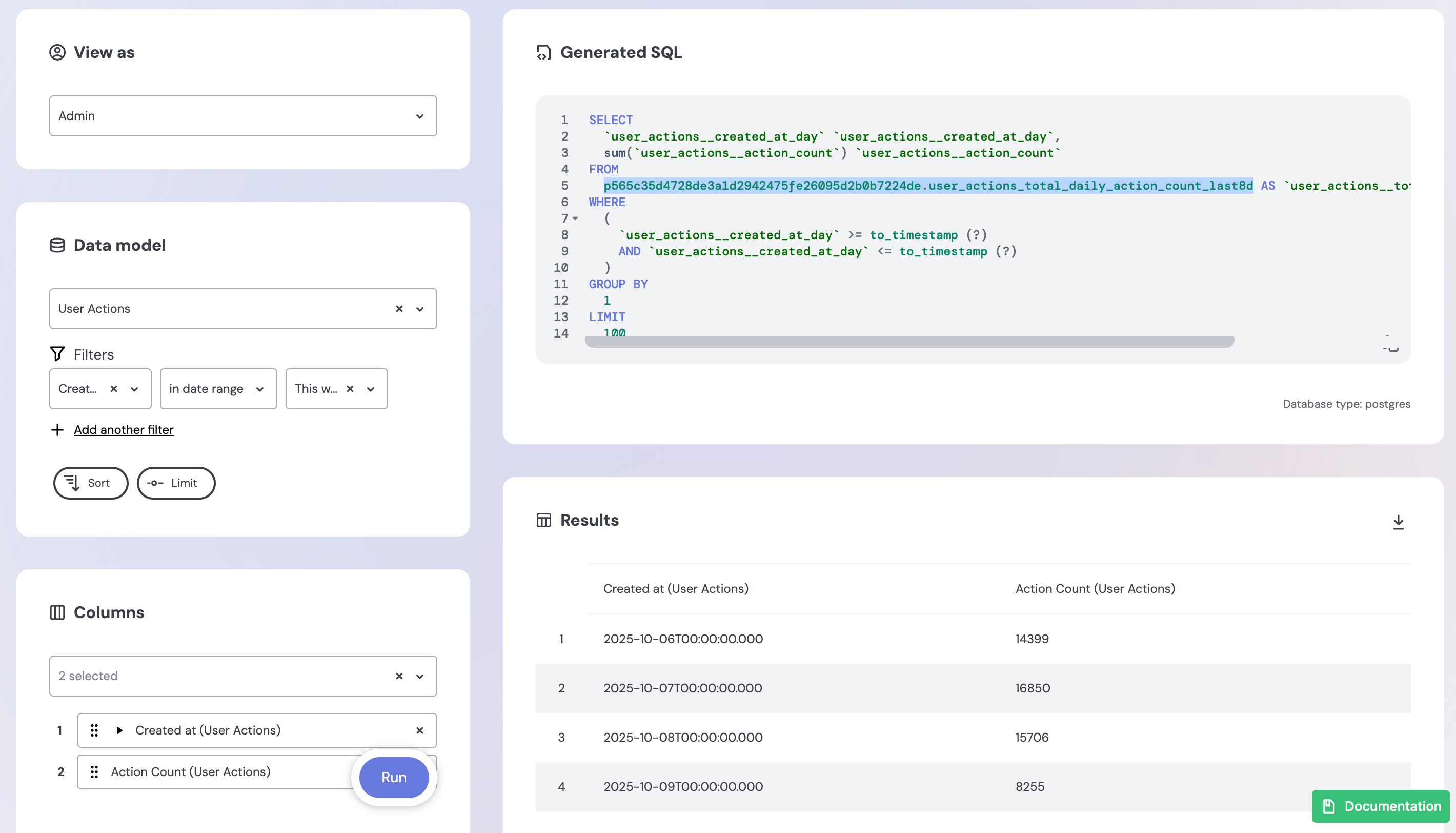
You can verify whether your pre-aggregation is being used by checking the generated SQL in the Embeddable Data Playground or in your Chart’s Query.

When a query uses a pre-aggregation, the SQL will reference the pre-aggregation table name instead of the underlying source table. For example:

FROM
p565c35d4728de3a1d2942475fe26095d2b0b7224de.user_actions_total_daily_action_count_last8d AS `user_actions__total_daily_action_count_last8d`

Things to notice:

The p<hash>.<pre_aggregation_name> pattern indicates the query is pulling data from the pre-aggregation rather than the underlying base table.
The hash prefix (e.g., p565c35d4728de3a1d2942475fe26095d2b0b7224de) is automatically generated using your workspace id, model version, security context and environment.

In the Data Playground

In the Embeddable Data Playground (opens in a new tab), the generated SQL preview will show the pre-aggregation table name in the FROM clause. This confirms that your query is using the pre-aggregated table.

In your Embeddable chart

If you’ve built an Embeddable that uses a dataset containing a pre-aggregation, you can confirm it’s being used by inspecting the chart’s SQL.

In the video below, you’ll see that the TableChart we created shows the same FROM clause pattern in its query, confirming that the chart is using the pre-aggregation rather than querying the base table directly.

Why do queries sometimes not use my pre-aggregations?

Importantly, if you want a query to use pre-aggregations, rather than hit your database, it must match exactly one pre-aggregation (even if you have defined multiple in your models). A query cannot combine the results of multiple pre-aggregations, or combine a pre-aggregation with data from your database. Any given query must be fully answerable from a single pre-aggregation, otherwise the query will always skip pre-aggregations and go straight to your database (you can see detailed docs on the matching algorithm here (opens in a new tab)).

Let’s look at some common examples where people get tripped up:

All query dimensions, measures and filters must be in the pre-aggregation
Time filters must match the requested granularity
If measures aren’t “additive”, this can cause cache-misses

Examples follow below.

1. All query dimensions, measures and filters must be in the pre-aggregation

Given a model with the following “count_by_countries” pre_aggregation:

cubes:
  - name: customers
    sql_table: public.customers
  
    dimensions:
        - name: id
          sql: id
          type: number
          primary_key: true
        - name: country
          sql: country
          type: string
        - name: signed_up_at
          sql: created_at
          type: time
          
      measures:
        - name: count
          type: count
          title: "Number of Customers"
   
      pre_aggregations:
        - name: count_by_countries
          measures:
            - CUBE.count
          dimensions:
            - CUBE.country

the following (or similar) SQL will be run against your database to generate the pre-aggregation:

SELECT
  "customers".country "customers__country",
  count("customers".id) "count"
FROM
  public.customers AS "customers"
GROUP BY
  1
ORDER BY
  2 DESC

which, in turn, will lead to the following pre-aggregation (or similar) being cached:

customers__country	count
United States	102
Australia	64
Germany	48
Canada	30
Belgium	5
…

That means that any of the following data queries can (and will) be served by this pre-aggregation (rather than going to your database):

Count by country:

{
    "query": {
        "dimensions": [
            "customers.country"
        ],
        "measures": [
            "customers.count"
        ]
    }
}

Cube can use all the columns and rows from the pre-aggregation above to serve this query, so it will use the pre-aggregation and it won't go to your database.

Count customers:

{
    "query": {
        "dimensions": [],
        "measures": [
            "customers.count"
        ]
    }
}

Cube can sum up the “count” column from the above pre-aggregation, so will use the pre-aggregation to serve this query.

Count US customers:

{
    "query": {
        "measures": [
            "customers.count"
        ],
        "filters": [
            {
                "member": "customers.country",
                "operator": "equals",
                "values": [
                    "United States"
                ]
            }
        ]
    }
}

Cube will take the “count” from the “United States” row from the pre-aggregation.

Countries with more than 30 customers:

{
    "query": {
        "dimensions": [
            "customers.country"
        ],
        "measures": [],
        "filters": [
            {
                "member": "customers.count",
                "operator": "gt",
                "values": [
                    "30"
                ]
            }
        ],
        "order": [
            [
                "customers.country",
                "asc"
            ]
        ]
    }
}

Cube will filter the pre-aggregation by the “count” column in the pre-aggregation and then sort the results by the “customers__country” column.

Any queries, however, where one or more of the dimensions, measures or filters in the query are not available in a pre-aggregation, will skip the pre-aggregations and hit the database instead.

For example this query:

{
    "query": {
        "dimensions": [
            "customers.id"
            "customers.country"
        ],
        "measures": []
    }
}

is asking for the “id” and “country” dimensions. This “country” dimension is in our pre-aggregation, but the “id” dimension is not. Cube will therefore go to your database instead to serve this query:

SELECT
  "customers".id "customers__id",
  "customers".country "customers__country"
FROM
  public.customers AS "customers"

because Cube can only use a pre-aggregation if it can, by itself, fully serve the given query.

2. Time filters must match the requested granularity

You can include time_dimension in your pre_aggregations (additionally to measures and dimensions) like so:

cubes:
  - name: customers
  
    ...
 
    pre_aggregations:
 
      - name: count_by_week
        measures:
          - CUBE.count
        time_dimension: CUBE.signed_up_at
        granularity: week
 
      - name: count_by_month
        measures:
          - CUBE.count
        time_dimension: CUBE.signed_up_at
        granularity: month

These two pre-aggregation will lead to the following SQLs (or similar) to be run against your database:

SELECT
  date_trunc('week', "customers".signed_up_at) "customers__signed_up_at_week",
  count("customers".id) "customers__count"
FROM
  public.customers AS "customers"
GROUP BY
  1

and

SELECT
  date_trunc('month', "customers".signed_up_at) "customers__signed_up_at_month",
  count("customers".id) "customers__count"
FROM
  public.customers AS "customers"
GROUP BY
  1

respectively. The results will be cached as pre-aggregations.

Notice how the time_dimension in the pre_aggregation also takes a granularity. In order to pre-aggregate by multiple granularities you must define a separate pre-aggregation for each granularity (like we’ve done in the "customers" model above).

For any incoming queries, Cube will try to find a pre-aggregation that can fully serve its dimensions, measures and filters (including timeDimensions).

Examples:

Count by month:

{
    "query": {
        "measures": [
            "customers.count"
        ],
        "timeDimensions": [
            {
                "dimension": "customers.signed_up_at",
                "granularity": "month"
            }
        ]
    }
}

This query perfectly matches the results in our “count_by_month” pre-aggregation, so Cube will use it.

Count of customers for last week:

{
    "query": {
        "measures": [
            "customers.count"
        ],
        "timeDimensions": [
            {
                "dimension": "customers.signed_up_at",
                "dateRange": "Last week"
            }
        ]
    }
}

Cube can filter our “count_by_week” pre-aggregation to the row from last week in order to serve this query.

Yesterday:

{
    "query": {
        "measures": [
            "customers.count"
        ],
        "timeDimensions": [
            {
                "dimension": "customers.signed_up_at",
                "dateRange": "Yesterday"
            }
        ]
    }
}

Neither of our pre-aggregations can answer this query (as there isn't a "day" granularity and you can't derive "day" from "week" or "month"), so Cube will skip pre-aggregations for this query and get it instead from our database.

2024:

{
    "query": {
        "measures": [
            "customers.count"
        ],
        "timeDimensions": [
            {
                "dimension": "customers.signed_up_at",
                "dateRange": ["2024-01-01", "2024-12-31"]
            }
        ]
    }
}

We don’t have a “year” pre-aggregation, but Cube is clever. We have a “month” pre-aggregation, and Cube can use that to sum up the counts for each month in 2024, and thus Cube will hit our “count_by_month” pre-aggregation to serve this query.

3. If measures aren’t “additive”, this can cause cache-misses

Above we have described multiple situations where Cube will serve an incoming data query, not just by returning a subset of the rows in the pre-aggregation, but by actually aggregating the counts from the rows.

E.g. in the last example above, Cube will calculate the number of customers for 2024 by summing up the counts for the 12 months of 2024. This works because measures of type “count” are “additive”. i.e. if you were to query your database directly for a count of customers who signed up in 2024, it will return exactly the same number as if you asked for the counts of each month in 2024 and sum them together.

Additivity is “a property of measures that determine whether measure values, once calculated for a set of dimensions, can be [accurately] further aggregated to calculate measure values for a subset of these dimensions” (source (opens in a new tab)).

The only additive measures are:

All other measures (avg, (opens in a new tab) count_distinct (opens in a new tab), etc.) are not:

avg calculates the average of a set of numbers. If January has three numbers: 3, 5 and 4 (which gives an average of 4) and February has just one number: 2 (whose average is obviously 2), then the average of January and February should be (3+5+4+2)/4 = 3.5. But if all you know are the two averages, 4 and 2, there is no way to accurately derive the correct average (you could average 4 and 2 to get 3, but this is incorrect). Thus avg measures are not additive.
count_distinct counts, not the total number of something (say, total visitors to a shop), but the unique (or distinct) number of something (say, unique visitors). If there were 5 unique visitors in January and 3 unique visitors in February, it does not mean that were (5+3) 8 unique visitors in January and February. Some of these visitors may have visited in both January and February, so the actual number may be as low as 5 (but may be higher). Thus count_distinct measures are also not additive.

And so, because Cube cares about giving correct numbers back, if your pre-aggregation is using non-additive measures (like avg and count_distinct) then it can still use the pre-aggregation if the query can be answered by returning a subset of the rows from the pre-aggregation, but if it would require aggregating them together in some way then it can’t use the pre-aggregation, and Cube will choose to skip the pre-aggregation and go to your database instead.

Workarounds for non-additive measures

You may be wondering: what if I want to use pre-aggregations for non-additive measures like avg and count_distinct?

There are a few workarounds:

avg is, in the end, just a calculation of a total divided by a count. Both a total and a count are additive, so you can separate the calculation into two additive measures and then calculate the average dynamically (notice that average_price below is purposefully not part of the pre-aggregation):

cubes:
  - name: customers
  
    ...
    
    measures:
      - name: total_price
        sql: price
        type: sum
      - name: count
        type: count
      - name: average_price
        sql: {total_price} / {count}
        type: number
 
    pre_aggregations:
      - name: price_and_count
        measures:
          - CUBE.total_price
          - CUBE.count

count_distinct is not additive (as explained in the previous section) but Cube has introduced a useful measure type called count_distinct_approx which tries to approximate the number of unique (distinct) values (learn more here (opens in a new tab)). It is useful if exact numbers are not essential and a rough estimate is sufficient.

Just bear in mind:
- the more rows from a pre-aggregation that you’re combining, the worse the approximation will be (e.g. if you’re calculating 2024 by aggregating 365 separate days of a count_distinct_approx measure, please don’t expect the result to be very accurate).
- unfortunately not all database types support count_distinct_approx. Check your specific database (e.g. here (opens in a new tab) you can see that MySQL doesn’t support it)
And finally, you can use non-additive measures in pre-aggregations confidently as long as your queries match the row granularity of your pre-aggregations perfectly. E.g. if your pre-aggregation shows count_distinct by week and your query requests that count_distinct measure for a particular week, Cube will use the pre-aggregation and return a perfectly accurate number.

Refreshing pre-aggregations

Now that we’ve added pre-aggregations to the model, the next step is deciding how to keep the data fresh. This is done with the refresh_key (opens in a new tab) property, which controls when Cube rebuilds a pre-aggregation.

Default refresh key

If you don’t define a refresh_key (opens in a new tab), Cube refreshes the pre-aggregation once per hour. This is a sensible default for most use cases, but you can override it if your data changes more or less frequently.

Refreshing on an interval

For predictable schedules, use the every property. This lets you define how often Cube should rebuild the pre-aggregation:

    pre_aggregations:
      - name: customer_countries
        dimensions:
          - CUBE.country
        refresh_key:
          every: 1 day

In this example, the pre-aggregation is refreshed once per day. This accepts time expressions like 1 second, 30 minutes, 2 hours, 1 day, 1 week, 1 month, 1 year.

For example every: 30 minutes or every: 2 hours.

You can also be more precise with a CRON string:

    pre_aggregations:
      - name: customer_countries
        dimensions:
          - CUBE.country
        refresh_key:
          every: "0 8 * * *"

This runs every day at 08:00. See the supported CRON formats (opens in a new tab) for more options.

Refreshing with SQL

Sometimes you only want to rebuild a pre-aggregation when the source data changes. In that case, use the sql property to define a query that checks for updates:

    pre_aggregations:
      - name: customer_countries
        dimensions:
          - CUBE.country
        refresh_key:
          sql: SELECT MAX(created_at) FROM public.customers

As we haven’t defined every, so when using the sql parameter the default interval is 10 seconds for every property. If the result changes, the pre-aggregation is refreshed.

Combining SQL with an interval

You can also combine SQL with your specific time interval. This lets Cube check for changes on a schedule:

    pre_aggregations:
      - name: customer_countries
        dimensions:
          - CUBE.country
        refresh_key:
          every: 1 hour
          sql: SELECT MAX(created_at) FROM public.customers

In this example the query every hour. If the result has changed since the last run, the pre-aggregation is refreshed.

💡

You can’t combine a CRON string with sql in the same refresh key. Doing so will cause a compilation error.

Performing joins across cubes in your pre-aggregations

All the examples so far have shown pre-aggregations using just the dimensions and measures from the cube in which it is defined. This is, however, not a requirement at all. You can easily define a pre-aggregation that uses dimensions and measures from multiple cubes, as long as the appropriate joins have been defined.

E.g. here you can see our pre_aggregation uses two dimensions (”make” and “model”) from the “vehicles” cube:

cubes:
  - name: person
  
    ...
      
    joins:
      - name: vehicles
        sql: "{CUBE}.id = {vehicles}.owner_id"
        relationship: one_to_many
      
    pre_aggregations:
      - name: person_vehicles
        dimensions:
          - CUBE.full_name
          - vehicles.make
          - vehicles.model
        measures:
          - CUBE.count
        time_dimension: CUBE.created_at
        granularity: day

Indexes

To get the best performance out of your pre-aggregations you will likely want to define indexes too.

Cube recommends "for most queries, there should be at least one index that makes a particular query scan very little amount of data”. You can read all about indexes here (opens in a new tab).

Handling incremental data loads

Sometimes your source data is updated incrementally for example: only the last few days are reloaded or updated while older data remains unchanged. In these cases, it’s more efficient to build your pre-aggregations incrementally instead of rebuilding the entire dataset.

Using the customers cube example:

pre_aggregations:
  - name: daily_count_by_countries
    measures:
      - CUBE.count
    dimensions:
      - CUBE.country
    time_dimension: CUBE.signed_up_at
    granularity: day
    partition_granularity: day
    build_range_start:
      sql: SELECT NOW() - INTERVAL '365 day'
    build_range_end:
      sql: SELECT NOW()
    refresh_key:
      every: 1 day
      incremental: true
      update_window: 3 day

Things to notice:

Most queries focus on the past year, so we limit the build range to 365 days using build_range_start and build_range_end. Learn more here (opens in a new tab).
partition_granularity: day splits the pre-aggregation into daily partitions, making it possible to refresh only the days that change instead of rebuilding the whole year.
Partitioned pre-aggregations require both a time_dimension and a granularity. See the Cube docs on supported values (opens in a new tab).
With incremental: true and update_window: 3 day, Cube refreshes only the last three partitions each day. Learn more about update_window (opens in a new tab) and incremental (opens in a new tab) .

💡

Without update_window, Cube refreshes partitions strictly according to partition_granularity (in this case, just the last day).

Next Steps

The next step is to setup Embeddable’s Caching API to refresh pre-aggregations for each of your security contexts.

In-memory cache Caching API